|
Introduction Demos with Positive Impact is an NSF
project to develop a web-based collection of effective instructional
demonstrations and to connect this resource to mathematics instructors. This article provides an update on the
project’s progress and showcases some of the demos that have been added within
the last year. Demos with Positive
Impact—An Ongoing Project Demos with Positive Impact was founded in
late 1999 as a project to develop a web-based collection of resources for
teaching mathematics. Funded by an NSF
proof-of-concept grant, the focus is on instructional demonstrations that we or
our colleagues have found to be useful and effective classroom tools. The project has a broad scope, encompassing
topics from secondary to undergraduate mathematics. In contrast to projects or lab activities for
students, demos are designed with the instructor in mind. Thus, the project goal is to provide a
collection of resources that the instructor can use to facilitate learning. The demos within
the collection are adaptable to a variety of learning styles and teaching
environments. Efforts are ongoing to
provide versions of the demos for a variety of technology platforms, including
platform-independent variations that run in a web browser. To date, the Demos with Positive Impact web site has
had visitors from countries such as Japan, China, Singapore, Australia, New
Zealand, Czech Republic, Netherlands, Sweden, just to name a few. Additionally, the audience has varied from
middle and high school instructors to community colleges and four-year colleges
and universities. A sub-collection of
the demos in the site has been featured in MathDL’s Digital Classroom Resources. Recently, the site was awarded distinction by
the Eisenhower National Clearinghouse as one
of the Digital Dozen for October, 2002. In the remainder
of this article we showcase some of the recent additions to the Demos with
Positive Impact collection and invite readers to contribute to the project as
end-users and by providing feedback. Enlightening Volumes: Curve Fitting to Approximate Volumes
This
demo is appropriate for calculus courses where volumes of solids of revolution
are discussed. It can be presented in courses, such as linear algebra and
numerical analysis, where an emphasis on the curve-fitting aspect of the demo
are appropriate. Additionally, it can be extended to use in courses where
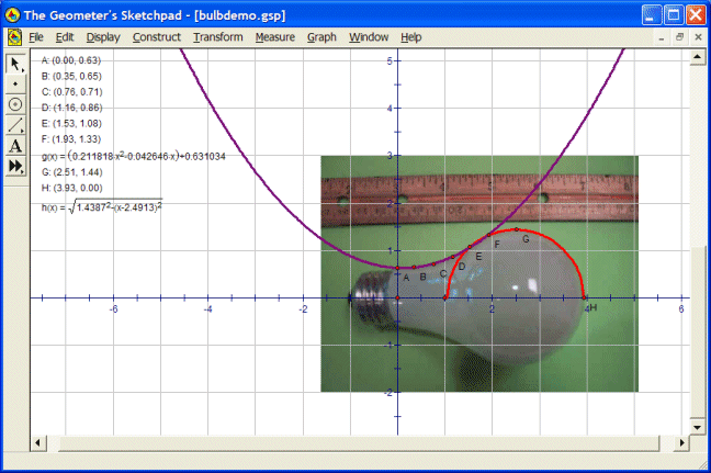
numerical quadrature techniques are discussed. The demo consists of two approaches. In one approach, a photograph of a light bulb is imported into Geometer’s Sketchpad and points along the edge are selected. The neck of the bulb appears much like a parabola. Using Geometer’s Sketchpad, points are selected and a quadratic regression determines the quadratic function that approximates the data points. In this demo, TI Interactive was used for the regression; alternatively a graphing calculator or computer software could be used. The round end of a bulb can be modeled using a circle. Using Geometer’s Sketchpad to collect three points along the round end, a circle with form
was found to
approximate the round end. Figure 1
illustrates the bulb together with the curves that approximate the shape. After the equations are determined, the
volume of the bulb is approximated using standard integration techniques for
solids of revolution (disk method). An alternate approach is to
use cubic splines to approximate the shape.
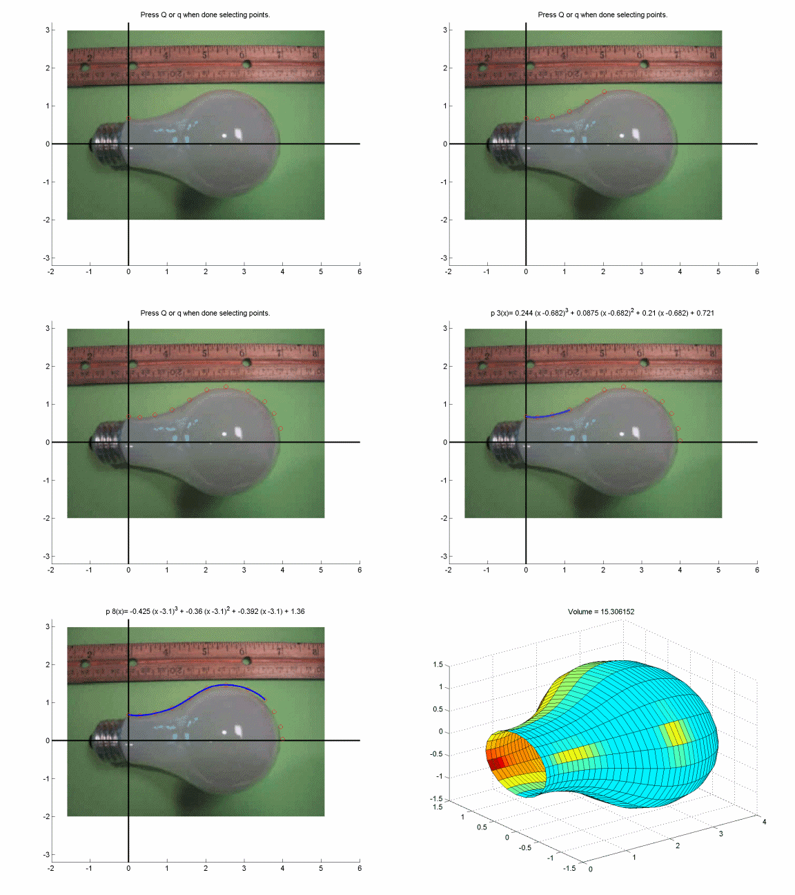
In this demo, the photograph was imported into MATLAB and points
collected along the edge of the bulb formed the basis of a cubic spline
approximation. The action of the MATLAB
routine (included with the demo) is illustrated in the animation in Figure 2. The animation shows how the points are
collected, the spline fit, and the resulting solid of revolution. This is a versatile demo that can be incorporated into mathematics courses at several different levels using a wide variety of technology tools. It is also a very nice example of a volume that would be difficult to directly measure and the power of the methods typically covered in calculus classes for computing volumes of solids of revolutions. The demo also illustrates appropriate uses of the various available technologies.
Figure 1. Parabola and Circle Fit to the Data. Figure 4. Cubic Spline Fit. Click on the picture to go to the animation.
Visualizations
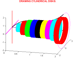
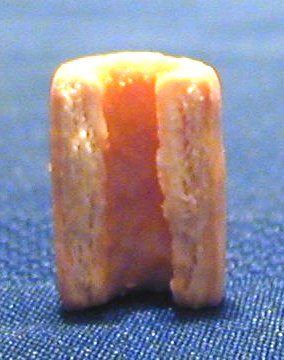
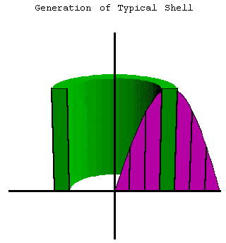
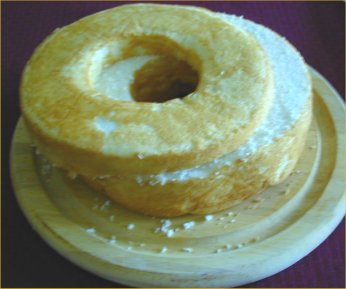
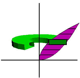
for Volumes of Solids in Calculus One of the most visited demos in the collection is actually a collection
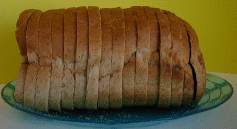
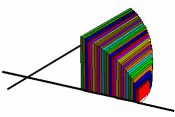
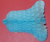
of demos that gives a comprehensive look at volumes of solids in calculus. Solids are modeled using physical objects and
the various techniques for approximating volumes are illustrated using
animations (both animated gif and mov formats).
Galleries that contain examples typical of textbook problems provide a
valuable tool for the study of volumes of solids in calculus. Figure 3 gives examples of the collection.
Figure 3. Volume Collection The purpose of this demo is to model and analyze the behavior of a resonant filter, including the solution of a second-order, constant coefficient differential equation, the notions of a transient and a steady state solution, and the idea of resonance. The resonant filter is a circuit element containing a resistor with resistance R, a capacitor with capacitance C, an inductor with inductance L and a voltage source. Its response can be modeled by a second-order, constant-coefficient, non-homogeneous second order differential equation
, where q(t) is the charge on the capacitor at time t and Vin(t) is the (known) voltage from the input source. The equation can be reforumlated in terms of current, i(t), using the relation that i'(t) = q(t). Differentiating, we obtain an equivalent equation in terms of the current in the circuit,
Let Vout(t) represent the voltage drop across the resistor. The relationship between the voltage and current is given by Vout(t) = R i(t). Thus, the second order differential equation equation, represented in terms of Vout is
A
program has been developed which takes as parameters the circuit elements,
the source, and the initial conditions. This program (included with
the demo) provides an interactive utility for a numerical simulation of the
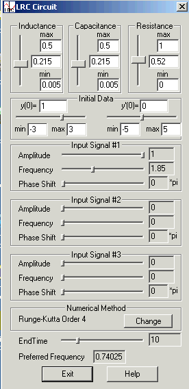
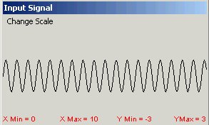
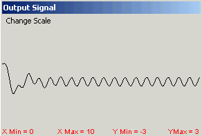
effect on the output by varying the parameters and the input signal. The program displays three components; the
control panel, a graph of the input signal, and a graph of the output signal,
represented by y(t). These are shown in Figure 4 for a particular
input function. This
demo provides four activities. A basic
demo involves simply illustrating the solution to an initial value problem that
models the resonant filter with one input signal. Holding all parameters
fixed except one, it is easy to investigate the effect on the output signal
from changing the value of one of the physical parameters. A second demo illustrates how solutions of a
second order differential equation with constant coefficients and a
sinusoidal forcing function decompose into two components—a transient
solution and a steady state solution. Simply sliding the bars for the
initial data shows quite clearly the presence of a transient solution that
depends on the initial data, and a steady state solution that is unaffected
by changes in the initial data. Two additional activities illustrate the
importance of resonance in electrical devices. Although resonance is
often undesirable in many mechanical systems, such as a spring mass system,
many electrical devices such as radios would not function properly without the
phenomenon of resonance. The program can
be used to simulate a primitive radio.
This is a very interesting example of resonance in action which is
relevant and real to students.
Constructing Equations from Word Problems Our experience as
mathematics instructors is that students often have a great deal of difficulty
with the formulation of mathematical models for physical situations described
in “word problems.” The purpose of this
demo is to provide a toolbox of visual aids for geometrically oriented word
problems. These visual tools are designed to help students to develop
equations that provide an algebraic model for the problem. These types of problems often form the basis
for related rates and optimization problems in calculus so while this demo can
be used in precalculus mathematics, it naturally leads to problem-solving at a
higher academic level. The demo provides a general outline of steps that apply to many verbal problems. The steps involved are illustrated with several examples. A collection of statements of geometrically oriented word problems is given together with visual demos (in the form of animations) that can be used within a lecture or assigned for students to use for practice. Users are expected to supply the algebra to accompany the situation. The animations can also be used as 'preview' material for optimization problems. Figure 5 gives a preview of illustrative examples.
Figure 5.
Examples from Word Problem Demo. An Invitation to Participate We invite you to participate
in the Demos with Positive Impact
project by sending us ideas that you have found to be successful for getting
students’ attention and helping them to understand mathematical concepts. We recognize that faculty members often are
not encouraged nor rewarded for activities related solely to development of
pedagogical tools. While we cannot pay
contributors for ideas, we do provide a mechanism by which mathematics
instructors can get some recognition for innovative teaching strategies. We invite you to visit the Demos with
Positive Impact web site for an on-line opportunity to contribute to the
project. In addition, we welcome
feedback on the collection or on individual demos within the collection.
Acknowledgements.
Partial support for this work was provided by the National Science
Foundation’s Course, Curriculum and Laboratory Improvement Program under grant
DUE-9952306. Enlightening Volumes: Curve Fitting to Approximate Volumes was contributed by Judy O’Neal, Visualizations for Volumes in Calculus demo collection was contributed by David R. Hill, The Resonant Filter was contributed by Michael O’Leary, Constructing Equations from Word Problems was contributed by David R. Hill,
|


 .
. .
. 