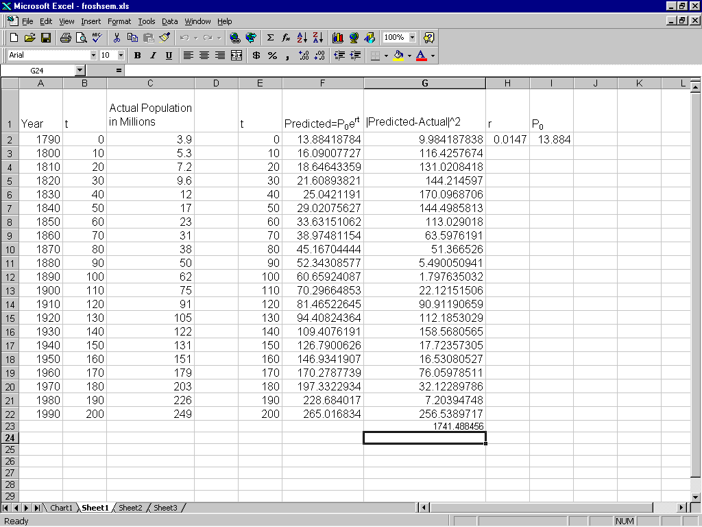
Figure 1: Setting up Exponential Regression
Most math majors have some exposure to regression in their studies. Usually, this exposure is limited to linear regression, polynomial regression and perhaps exponential regression using least squares. With the advent of new technology, I think it is time to consider some alternatives. Using Excel and its built-in optimization tool called the Solver, it is possible to introduce other forms of regression (and reconsider some old ones). In this paper, we will discuss some of these regression problems.
In this section we consider exponential regression. We'll see that if we do exponential regression in the usual way, we get an answer that is not as good as it could be. Let's consider fitting an exponential function to the US census data taken from [1] and see what happens. First we will do the standard exponential fit and then we will compare the result we obtain using the Solver.
| Year | Population | Year | Population |
| 1790 | 3.9 | 1890 | 62 |
| 1800 | 5.3 | 1900 | 75 |
| 1810 | 7.2 | 1910 | 91 |
| 1820 | 9.6 | 1920 | 105 |
| 1830 | 12 | 1930 | 122 |
| 1840 | 17 | 1940 | 131 |
| 1850 | 23 | 1950 | 151 |
| 1860 | 31 | 1960 | 179 |
| 1870 | 38 | 1970 | 203 |
| 1880 | 50 | 1980 | 226 |
| 1990 | 249 |
Table 1: US Census Data
The usual method for fitting an exponential function, y = aebx, to data is to take logarithms of the y data and perform linear regression on the new data. This action was performed on the data above and the results are tabulated below.
| a | b | SSE |
| 5.73944 | 0.020834 | 24339.92 |
Table 2: Standard Regression Fit
We can fit the data by choosing a and b to minimize the sum of the squares of the errors without logarithms. Excel's optimization tool will do the hard work for us. In Figure 1, we see a spreadsheet set up to do regression on this data. We compute the squares of the residuals in column G and in cell G23 we have their sum. This is the quantity to be minimized. The values in cells H2 and I2 control this sum. Now we are ready to set up the Solver.

The Solver is called up from the tools menu. If you don't see it there, it may be for one of two reasons. The first reason is because it is not installed with the standard installation of MS Excel. In this case, you need to run the setup program again to install it (see [4]). Even if the Solver is installed, you need to make it accessible to the workbook you have opened. To do this, look under the tools menu for add-ins and click there. It should bring up a dialog box with all the add-ins that you have installed. Check the box for the Solver. Now we are ready to do some regression.

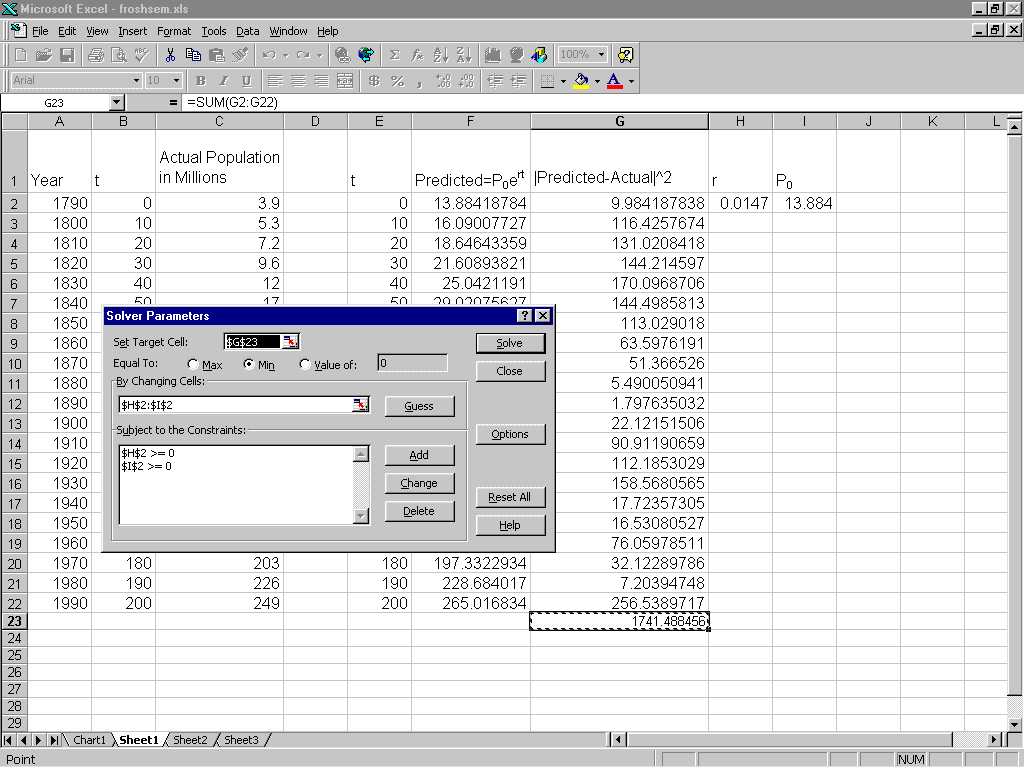
Once you have the Solver runnning, the first step is to set the target cell, i.e. the cell that has the value to be maximized or minimized (see Figure 2). For the problem illustrated the sum is in cell G23. Next you enter in the cells that control the target (H2 and I2). Finally you enter constraints, in this example the constraints are not necessary, but were entered for illustration purposes. When everything is set up, you hit the solve button and voila! Here is the fit given by the Solver:
| a | b | SSE |
| 13.884 | 0.0147 | 1741.49 |
Table 3: Regression Fit without Logs
Notice the difference between the two answers we have calculated. The SSE for the standard regression is much larger than that achieved by direct minimization. This type of result seems to be true for many types of nonlinear regressions [3].
Usually, when we are talking about regression we mean that we are minimizing the sum of the squares of the errors. Using the Solver, a person could easily compute other regression fits with a different measure of error. For example, instead of the usual least squares you could request a minimum of the sum of the absolute deviations or possibly the minimum maximum error. Let us try these different fits on the population data above. The following table has the coefficients determined by minimizing the different error measures mentioned above. We can see that there are some differences in the calculated fits. Other measures of the error could also be used.
| Type | a | b |
| Direct | 13.884 | 0.0147 |
| Logged | 5.7394 | 0.0208 |
| Absolute | 14.073 | 0.0148 |
| Minimax | 28.226 | 0.0102 |
Table 4: A Comparison of Several Regression Fits
Logistic regression is a topic that does not get much attention in the undergraduate statistics books. Partly because the computations needed to perform it are more complicated than other regressions. Using the Solver, logistic regression is no more difficult than any other to perform.
Logistic regression is different from regular regression because the dependent variable can be binary. This type of data is often gathered in medical studies. For example, a researcher may test individuals for the presence or absence of a disease and attempt to assign a probable risk. In the example that follows we examine some data on coronary heart disease taken from [2]and compute the logistic regression fit to this data. Age is the independent variable and the dependent data is binary with 1 indicating the presence of coronary heart disease and 0 indicating its abscence. We seek a function which fits this data and predicts in some sense the probability of CHD being present at a given age. One such function see [2] for details) is given by
| (1) |
The issue is how to detemine the parameters b0 and b1. Unlike regular regression problems, we cannot use least squares to estimate these parameters. The usual method of estimation is called maximum likelihood. In order to apply this technique, we must first construct a likelihood function. We estimate the parameters in our regression equation by choosing them to maximize the likelihood function we construct. Let
| (2) |
| (3) |
| b0 | b1 |
| -5.32351 | 0.11127 |
Table 6: Logistic Regression Fit
| Age | CHD | Age | CHD | Age | CHD | Age | CHD |
| 20 | 0 | 35 | 0 | 44 | 1 | 55 | 1 |
| 23 | 0 | 35 | 0 | 44 | 1 | 56 | 1 |
| 24 | 0 | 36 | 0 | 45 | 0 | 56 | 1 |
| 25 | 0 | 36 | 1 | 45 | 1 | 56 | 1 |
| 25 | 1 | 36 | 0 | 46 | 0 | 57 | 0 |
| 26 | 0 | 37 | 0 | 46 | 1 | 57 | 0 |
| 26 | 0 | 37 | 1 | 47 | 0 | 57 | 1 |
| 28 | 0 | 37 | 0 | 47 | 0 | 57 | 1 |
| 28 | 0 | 38 | 0 | 47 | 1 | 57 | 1 |
| 29 | 0 | 38 | 0 | 48 | 0 | 57 | 1 |
| 30 | 0 | 39 | 0 | 48 | 1 | 58 | 0 |
| 30 | 0 | 39 | 1 | 48 | 1 | 58 | 1 |
| 30 | 0 | 40 | 0 | 49 | 0 | 58 | 1 |
| 30 | 0 | 40 | 1 | 49 | 0 | 59 | 1 |
| 30 | 0 | 41 | 0 | 49 | 1 | 59 | 1 |
| 30 | 1 | 41 | 0 | 50 | 0 | 60 | 0 |
| 32 | 0 | 42 | 0 | 50 | 1 | 60 | 1 |
| 32 | 0 | 42 | 0 | 51 | 0 | 61 | 1 |
| 33 | 0 | 42 | 0 | 52 | 0 | 62 | 1 |
| 33 | 0 | 42 | 1 | 52 | 1 | 62 | 1 |
| 34 | 0 | 43 | 0 | 53 | 1 | 63 | 1 |
| 34 | 0 | 43 | 0 | 53 | 1 | 64 | 0 |
| 34 | 1 | 43 | 1 | 54 | 1 | 64 | 1 |
| 34 | 0 | 44 | 0 | 55 | 0 | 65 | 1 |
| 34 | 0 | 44 | 0 | 55 | 1 | 69 | 1 |
Table 5: Coronary Heart Disease as a Function of Age
We have examined several standard and nonstandard regression problems in this paper and seen how Excel can help to compute regression equations. Why use Excel at all when there are other packages available? The main reasons are:
For these reasons, I hope that you will consider using Excel the next time you teach regression.