Although knowledge of a spreadsheet is one of the essential tools for any college graduate,
colleges often find it difficult to devote a complete semester to teaching it. This is where the
sophistication of today's spreadsheets may come into play. They can be used in almost all fields,
in particular they are at home in the mathematical sciences domain. That is, one can teach
introductory college level mathematics using a spreadsheet as a tool. In this manner students
learn about the spreadsheet even though the spreadsheet itself would not be the primary objective
of the course.
Any of the most recent versions of the commercially available spreadsheets are equally capable of
performing such service. I have chosen Microsoft Excel for this purpose. Here are some of the
mathematical subjects that I tackle using Excel as the tool: polynomials and their properties,
quadratic equations and quadratic formula, solving equations by approximating their roots,
solving systems of two equations and two unknowns, optimization, linear programming,
trigonometric functions, exponential and logarithmic functions, binomial expansions and Pascal's
Triangle, normal and discrete probability distribution functions, and amortization.
In addition to the above mathematical concepts, one can use the programming capability of the
spreadsheet to include some programming concepts. For example Excel uses the Visual Basic
programming language for its macros. One can push this aspect as little or as far as such a course
allows.
To give some examples, I'll present a brief description of some of these topics.

The same technique can be used to solve any system of equations in two variables.
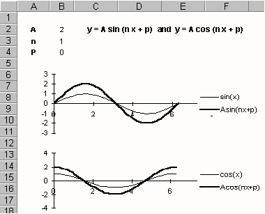 Y = A sin (n x + P)
Y = A cos (n x + P)
name three cells A, n, and P. Use
these names to generate the
function values over the interval
[0, 6.3] representing the interval
[0, 2]. Graph these two functions
next to the graphs of sin(x) and
cos(x). Now by entering different
values for A, n, and P we can
examine their effects on both
graphs. This method provides a
quick confirmation that the
parameter A sets the amplitude,
parameter n effects the period, and
parameter P corresponds to the phase shift.
One can even show the graphical proofs of equalities such as
sin(-x + /2 ) = cos(x)
cos(-x + /2 ) = sin(x)
by setting A = 1, n = -1 and P = PI()/2
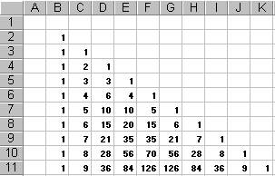
The function C(n, m) in Excel returns the value of "n choose m". That is,
![]()
The binomial expression (x + y) n can be represented by
(x + y) n = C(n, 0) xn + C(n, 1) xn - 1 y + C(n, 2) xn - 2 y2 + ... + C(n, n) yn
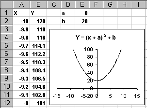 The relationship between the function f(x) and
its linear transformation f(x + a) + b can be
investigated by graphing both functions for
variety of values for a and b. To do so, name
two cells a and b respectively. Generate x and
y values for your function over a set interval.
The y values for the function f(x + a) + b are
evaluated directly. For example if f(x) = x 2,
enter the formula = (x + a)2 + b for the first y
value and copy it to the entire y range. When
changing the values of a and b, graph responds
accordingly. This visualization technique helps
students to understand linear transformations
by examining variety of quick examples.
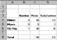 Susan has set aside $100 for her monthly entertainment. If a
dinner costs $15 with the satisfaction rate of 35, a movie costs $7
with the satisfaction rate of 15, and a skiing trip costs $40 with
the satisfaction rate of 90. How should she spend her
entertainment money to maximize her satisfaction?
To set this problem up, enter the labels as shown. Enter
appropriate formulas in the Price and Satisfaction columns. For instance, enter B4 * 15 in C4,
B4 * 35 in D4, and C4 + C5 + C6 in C8. Use the Solver to maximize the cell D8 which
represents the total satisfaction based on the following constraints:
B4 = Integer
B4 >= 0
B5 = Integer
B5 >= 0
B6 = Integer
B6 >= 0
C8 <= 100
This will produce values 4, 0, and 1 for the number of dinners, movies, and ski trips, respectively.
Reference
Golshan, Bahram Problem Solving with Microsoft Excel, Lycoming College, Williamsport PA,
1997.