Exploring Discrete Mathematics with MAPLEV:

Instant Insanity Meets Computer Algebra

Shepherd College Shepherdstown, WV 25443

skunyosy@shepherd.wvnet.edu

0. INTRODUCTION

The major themes of a first course in discrete mathematics are generally logic and proofs,induction and recursion, counting techniques, algorithms and their analysis, elementary graph theory,applications and modeling. Among the goals of this course are understanding the concepts of proofs and improving mathematical reasoning and problem solving skills.

Solving any challenging problem often requires putting oneself in the right position to gain some crucial insight. To be an effective problem solver, one needs to consider alternatives, to experiment, to conjecture, to test, and to analyze the results. In short, an exploratory attitude is an essential ingredient of problem solving skills.

Computer Algebra Systems encourage the exploratory attitude in students by providing easy to use graphical and numerical capabilities, as well as symbolic capabilities. Shifting the burden of tedious computation to a machine allows the students more time to concentrate on how to approach a problem, to delineate sub-problems, to consider alternatives, and to experiment. This paper is intended to provide some examples of how Maple, a Computer Algebra System that provides a mathematical problem solving and programming environment, can be used to challenge our students with conceptual understanding, problem solving, and explorations, using problems and concepts from topics in discrete mathematics.

SETS, SEQUENCES, AND LOGIC

1.1 Set, and Sequence

A set is a collection of distinct objects; it is also an object itself. Sets are useful in helping us understand the relationships that hold among mathematical concepts. Set theory is a convenient and precise language with which to express complicated mathematical relationships.

In Maple, a set is represented by a list of objects separated by commas, and enclosed between a pair of curly brackets, the same way we do in Mathematics. Unlike a tuple or a finite sequence of numbers, a set is a list that is un-ordered and has no repetitions. To distinguish between a set and a tuple, or ordered list, Maple uses the square brackets to represent the latter. For example {a,b,c,d} is a set of four elements. But [a,b,c,d] is a 4-tuple.

1.2 Inductive Definition

One way to describe a set is to define properties for its member. Inductive definition is frequently used in mathematics and computer science to define the elements of a particular set. An assignment that has students write a Maple code to form a set based on its inductive definition will help the students develop dynamic mental images associated with the set and the properties of number system. An inductive definition of a set S consists of three steps: basis, induction and closure. The following example gives an inductive definition for defining non-negative even integers.

	Basis:           0  is in E
	Induction:       If  n  is in E, then  n + 2 is in   E
	Closure:         Nothing else  are in E.

1.2.1 Maple code for set of non-negative even integers

>  evennum :=proc(n) options remember;
>  if n = 1 then 0 else  evennum(n-1)+2   fi:  end;

The function evennum(k) returns the kth non-negative even number. For example, evennum(3) returns 4.

If we want to print out a list of non-negative even integers, we can use a simple for-loop:

	> for i from 1 to N do print(evennum(N)); od:

	(assuming N has been previously assigned a value.)

To form a set of (a finite number, 50 say) of non-negative integers, we use the following code.

	> evenset := NULL: for i from 1 to 50 do

	> evenset := evenset, evennum(i) od:

	> print(evenset);

1.2.2 Examples of assignments for students

Write a Maple code to construct the following sets based on Inductive definition.

	(a) Set of the Fibonacci numbers.

	(b)   Set of  positive odd  integers.

	(c)   Set of negative even integers.

	(d)   Set of even integers.

	(e)   Set of composite  numbers between  2 and 100.

1.3 Logic
The fact that a set has no repeated members can be used to our advantage in the study of Logic and especially in the proofs of validity of an argument. For example, to show the expression (not p or q) is equivalent to (p implies q), we have to show that the expression (not p or q) = (p implies q) is true for all combinations of truth values of p and q.

This can be done in two different ways on MAPLE.

Use MAPLE nested for-loop to print out the truth values of the expression for all combinations of truth values of p and q.
Compute the truth-value for each combination and storethe result in a set. This method will return {true} if the expression is a tautology and {false} otherwise.

1.3.1 Maple code for (1):

	>  with(logic):

	>  S := [true, false];

	>  for p in S do

	  >  for q in S do

	    >  print(p,q,  bequal((not q)&implies(not p) ,(p &implies q)):

	>  od: od:

The following output is obtained:

               true, true, true
                        true, false,true
                       false, true, true
                       false, false,true

1.3.2 Maple Code for (2)

 > with(logic):

> s := {}: # initialize the set s

> S := [true,false]:

> for  p in S do for q in S do

> s:= {op(s), bequal((not q)&implies(not p) ,(p &implies q))}:

> od: od :

> print(s);

Output:
                       {true}

2. MATRIX AND GRAPH THEORY

2.1 Power of an Adjacency Matrix of a Graph.

Matrix Algebra has applications in many areas of mathematics, and especially in Graph Theory. A graph is a series of vertices connected by segments called edges. The term "graph" normally means a simple graph, in which no loops or multiple edges are allowed. A graph or multigraph may be represented by an matrix whose entries are the number of edges that connect one vertex to another. Such matrix is also known as an Adjacency Matrix.

2.2 Problem for Investigation with MAPLE

The objective of the problem and assignments below is to have students investigate the relationship between the powers of the matrix representing a graph and the number of paths of a given length between its two vertices.

2.2.1 Problem

Construct the matrix representing a multi-graph with 3 vertices and 4 edges. There are two edges between the first vertex and the third vertex, and one each between the second and the third, and the second and the first. (Call the first vertex A, the second B and the third C.)
Draw the graph represented by the matrix above.
How many paths of length 2 are there from vertex A to vertex B? Of length 3?
Enter the matrix in Maple and call it M. Compute M*M and M*M*M. What does the (i,j)entry of M*M represent? Of M*M*M?
Repeat (2) and (3) using a different graph .
Make a conjecture as to what the (i,j) entry of M^n represent. Prove your conjecture.

2.2.2 Students' discovery:

When the original matrix is squared, the entry gives the number of paths composed of two edges connecting two vertices. When cubed, the entry gives the number paths composed of three edges connecting two vertices.

3. Applications of Graph theory and Adjacency Matrices

If the graph represents airline flights between cities, the process above gives useful information about the number of routes with one stop, two stops, and so on. Doing matrix computations by hand can be tedious and often error prone. Using Maple, on the otherhand, helps remove this drudgery and encourages the student to investigate many examples of graphs before forming a conjecture.

On the lighter note, the entertaining aspect of graph theory lies in its usefulness for analyzing certain kinds of games and puzzles. The following problem is based on the "Instant Insanity" puzzle in Chatrands' Graphs as Mathematical Models. [3]

3.1 The multi-colored cubes problem

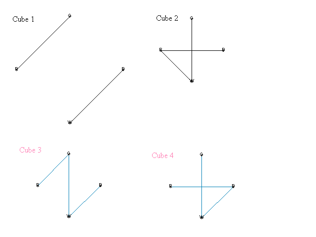
The "instant insanity" puzzle, a trade name used by the Parker Brothers Game Company, consists of four cubes with faces colored with four colors (red, blue, green, and white in this example). The object of the puzzle is to stack these cubes in a column so that each side (front, back, left, and right) of the stack shows each of the four colors. A graph with four vertices labeled B, G, R, W (for blue, green, red, and white) can be used to represent each cube; there is an edge between two vertices if the two colors are on the opposite sides of the cube, and a loop at a vertex if the opposite sides have the same color.

The graphs of the four cube are:

Graphs for the four cubes are entered in  MAPLE as follows.

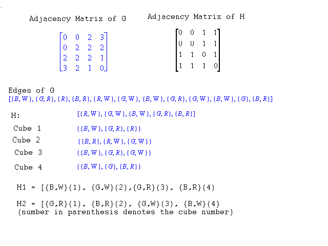
 > cube1 := graph([B,G,R,W], {{R,R},{B,W},{G,R}} ):

 > cube2 := graph([B,G,R,W],{{B,R}, {R,W},{G,W} })

 > cube3 := graph([B,G,R,W],{{B,W},{G,R},{G,W} })

 > cube4 := graph([B,G,R,W],{{B,R},{B,W},{G,G}}):

If we superimpose the four graphs together a multi-graph, G, is formed. The problem will be solved if we can find two disjoint subgraphs of G, each of order 4 ,one for front-back and the other for left-right configurations. The two subgraphs must not share edges since a given edge cannot represent both front-back and side-side at the same time. And each subgraph must contain exactly one edge from each cube.

Instead of using the diagram of G to extract two required sub-graphs, a task mostly done by trials and error, we can write Maple code to form the union of the graphs of the four cubes and extract a simple subgraph H, using Maple's gsimp() function. If it is possible to extract two order-4 edge-disjoint subgraphs of H then the problem is solved. By examining the adjacency matrix of H, we can also determine whether the puzzle is solvable or not.

We now examine the adjacency matrices of G and its maximal subgraph H together with the lists of edges in G, H, and the four cubes.

    One possible solution for the above problem is :

		FRONT   BACK		LEFT    RIGHT

Cube 1            B       W 		G       R
Cube 2            W       G          	R       B               
Cube 3            G       R            	W       G
Cube 4            R       B            	B       W

For MAPLE worksheet example, send e-mail to skunyosy@shepherd.wvnet.edu

4. CONCLUSION

Maple is a very powerful tool for doing mathematics and an efficient learning tool, if used properly. As illustrated in the above examples, Maple can handle a lot of quot;grunge' work that is tedious and error prone when done by hand. Using Maple to do the busy work allows the students more time to investigate and to explore, and to look at more realistic problems.

5. REFERENCES.

Baxter, Nancy, Dubinsky, Ed, & Levin, Gary, Learning Discrete Mathematics with ISETL, Springer-Verlag, New York, 1988.
Book, David L. Problems for Puzzlebusters, Enigmatics Press, Washington DC.
Chatrand, Gary, Graphs as Mathematical Models, Wadsworth International Group, Belmont, California, 1977.
Jackson, Bradley W. & Thoro, Dmitri, Applied Combinatorics with Problem Solving, Addison-Wesley Publishing Company, New York 1990.
Small, Donald B. & Hosack, John M., Explorations in Calculus with a computer Algebra System , McGraw-Hill, New York 1991.