It was three years ago that my colleague, Tim Sipka, and I decided to begin incorporating computer algebra system (CAS) technology into our calculus program. We opted to use the CAS, not to supplant hand computation altogether as some good programs have done, but instead to supplement our existing traditional program. Our simple guiding goal, we decided, would be to try to find ways to use the new technology to help students understand the concepts of calculus better. After experimenting with a few systems, we chose Maple and began developing laboratory assignments which students would carry out in groups of two or three. Of the sixteen topics we've used Maple to teach, I've found that the ones which are most enhanced by the technology are the multivariable topics. In this paper, I share two of the laboratory activities we have used to teach them. Also, I share the results of a student opinion survey about our project.
The first of these is the topic of space curves. The purpose of the lab we wrote on this was to help students visualize three-dimensional curves by

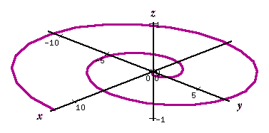
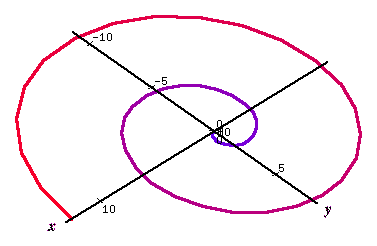
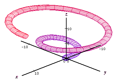
then the spiral will stretch up out of the plane. See Figure 2a. We want the students to see the projection of the curve in the xy -plane, so we rotate the z -axis forward (see Figures 2b and 2c) until our viewpoint is directly over the xy -plane (Figure 2d) and we see the same curve as when z was forced to be 0.
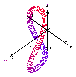
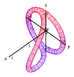
Maple has a feature called "tubeplot" which plots the curve as a hollow tube. See Figure 3. Notice how this feature especially helps in interpreting the apparent intersections of the curve. It is clear in this plot which portions of the curve are in front of others. We'll use this feature now to plot another space curve.
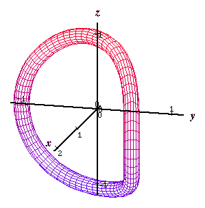
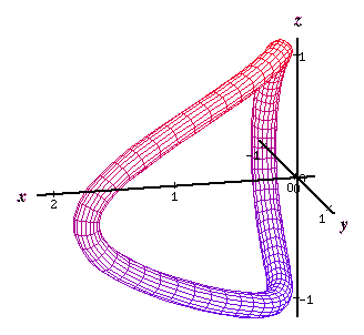
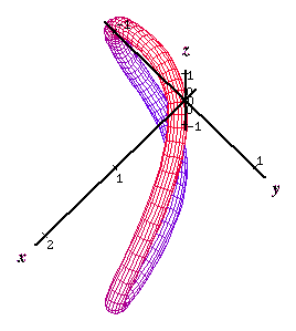
An advantage of using the CAS is that students can start analyzing some interesting curves right away--much earlier than we would have expected them to do just plotting by hand. One of the curves we have them analyze has parametric equations

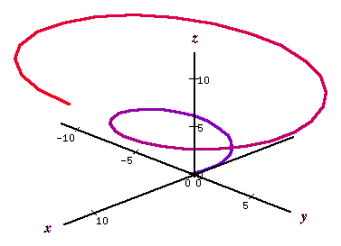
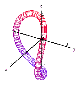
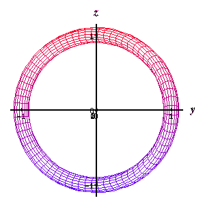
A tube plot of this curve is shown in Figure 4a. We tell the students to rotate the curve so that they are looking straight down each axis. Let's start by rotating the x -axis upward and to the right (see Figures 4b and 4c) until we see the projection of the curve onto the yz -plane (Figure 4d). As it should be, this is a circle.
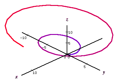
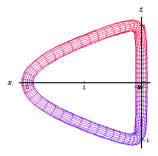
Now, back the original view (Figure 5a), and we'll rotate the y -axis upward and to the left (Figures 5b and 5c) until we see the projection of the curve in the xz -plane (Figure 5d). We can see in this projection that z is between -1 and 1 as it should be, and that x is between 0 and 2. (Actually, x is between about 0.0001 and 2.)
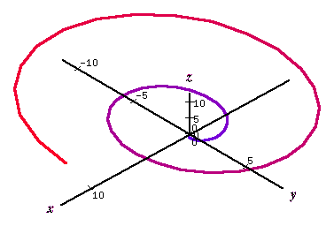
Finally, we'll rotate the z -axis forward (Figures 6a, 6b, 6c) until we can see the projection of the curve in the xy -plane (Figure 6d). As it should, y falls between -1 and 1, and x is between 0 (actually about 0.0001) and 2.
We feel that this kind of exercise really gives the students a better feel for the way these curves sit in space and that, after doing this lab, they are able to visualize a space curve reasonably well by inspection of the parametric equations.
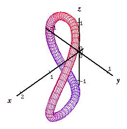
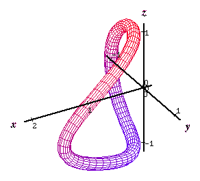
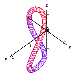
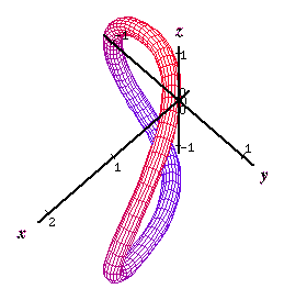
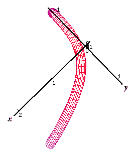
It's interesting to see what happens if we increase the domain of t from [-pi, pi] to [-2 pi, 2 pi]. This graceful curve is shown in Figure 7. We can see that, as t takes on larger absolute values, the x -coordinates become very small, so the curve hugs the yz -plane. The curve is traversed from the right-hand side near the y -axis (when t = -2 pi), upward and to the left.
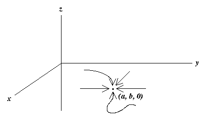
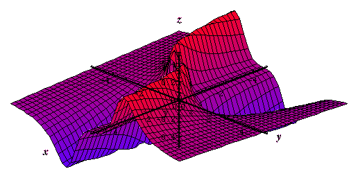
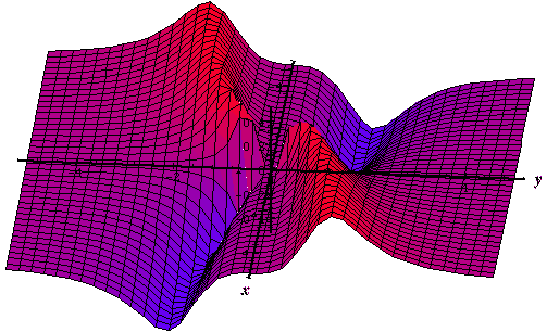
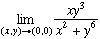
Probably the best spot of all that we've found to use a CAS is to teach the concept of limits of real-valued functions of two real variables. Before we turn them loose on the lab, we tell the students that the concept of limit is complicated by the requirement of path-independence. That is, the single-variable notion of approach from either side becomes approach from every direction and along every possible curve. See Figure 8. Typically, calculus text books include limit problems in which a function nears the same value along all lines of approach, but it tends to a different value along some curve of approach. The student is supposed to find such a curve by inspection. While this is a valid activity, another way is to use the graphics capability of a CAS--and especially the ability to rotate the surface--to help find such a curve or, at least, determine that there is probably one to be found. Here is a problem from our lab:
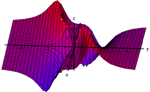
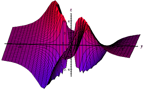
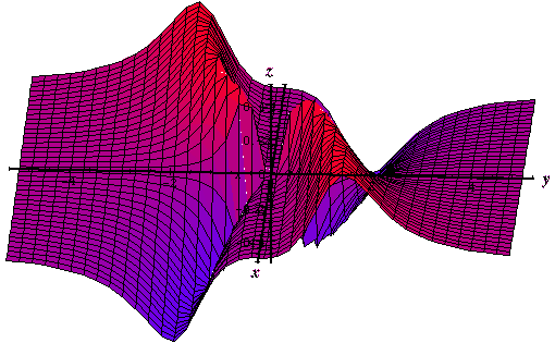
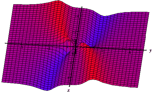
A plot of this appealing surface is shown in Figure 9a. Again, the activity is to look at the surface from many points of view. See Figures 9b and 9c. We can see that something fairly precipitous is happening near the origin, and that the function nears a different value along the ridge than it does along lines of approach to the origin. (It also tends to a different value along the trough, but we'll concentrate on the ridge.) To get a better look at the ridge, we'll rotate the z -axis forward. See Figures 9d, 9e, and 9f. We hope this leads students to recognize the ridge curve

(or, possibly, the trough curve) in the surface and then to
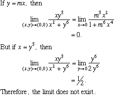
We find that the capability the CAS provides to graph and manipulate the surface gives students something concrete to associate with this analytic process.
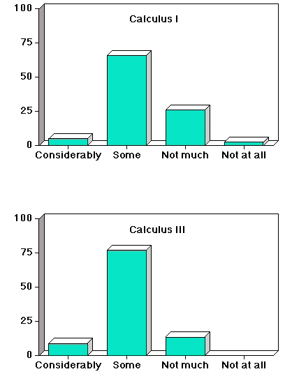
To learn whether the students thought things were going as well as we did, I surveyed a Calculus I class and a Calculus III (Multivariable Calculus) class. Among other things, I asked,
Do you believe that using Maple is assisting you in learning calculus?with possible responses
The results are shown in Figure 10. In Calculus I, 71% of the students thought that Maple was helping them to learn calculus. In the multivariable course, 86% thought that using Maple was helping them. So students are generally favorable and, in the multivariable course, highly so.
The survey confirmed my own suspicion that a CAS is particularly helpful in the multivariable course. Certainly, I'm convinced that this is the way to teach the course. I can't imagine teaching it now without a computer algebra system.
Acknowledgment:
I thank Myles McNally who helped me to format this paper in HTML.